Matching to estimate the causal effects of firing an NFL coach

Note: This post is a bit longer than usual. It’s part tutorial and part analysis. Feel free to jump to the conclusions, which are (I think) quite interesting. Additionally, the data and code are posted on Github.

The 2016 NFL regular season has ended, and with it has come the usual coaching carousel in which many franchises have opted to fire their head coach.

As of January 2nd, six of the league’s 32 teams have openings, with five of those coming by way of a fired predecessor (Denver’s retiring Gary Kubiak being the lone exception). But it’s not like 2016 is any type of outlier; roughly 4 coaches per year have been canned since the early 1980’s.

What’s interesting, though, is that despite the frequent, franchise-altering decisions made across the league, it’s mostly unknown whether or not this choice benefits longterm franchise prospects. (Postscript: Today, Brian Burke looks at the identical question here, finding similar answers to what I find below).  As one exception to the rule in soccer, one study found that sacking a manager in soccer offered no tangible benefit to the future performance of a club.

So, does firing a coach cause teams to improve?

The point of this blog post will be to look back at past firings, and to use some standard causal inference tools to help us identify if the choice of whether or not to fire a coach has been a helpful one.

A naïve approach

Estimating causes and effects when it comes to coach firings, unfortunately, is in no way straightforward.

The easiest strategy would be to compare the performance of franchises who fired their coaches in the seasons pre and post firings. For example, since 1982, the 130 teams who have fired their coach (using end-of-season firings) boasted an average improvement in winning percentage of 0.10, or the equivalent of about 1.6 games in a 16 game season. That’s a notable and statistically significant improvement.

Of course, that simple strategy is also a misleading one. The teams who got rid of their head coach only averaged about 5 wins per season prior to the firing, so on account of reversion towards the mean, we would’ve expected most of these teams to improve, anyways.

We can and should do better.

Potential outcomes

Let’s introduce some causal inference lingo.

In an ideal world we’d observe two outcomes, (i) the future performance of a team that fired its coach and (ii) the future performance of that same team that kept its coach. These are termed potential outcomes, and if we knew both potential outcomes, it would of course be easy to pick an optimal strategy.

Alas, short of building a time machine, knowing both potential outcomes is infeasible, and we’re only left with knowing the path chosen by each franchise. This is what’s known as the fundamental problem of causal inference; we want to be able to contrast an observed outcome with something that can’t be observed.

As it turns out, this also makes causal inference a missing data problem – the missing data is the missing potential outcome. In our case, for a team that fired its coach, the missing outcome is the path that would have been observed had that team kept its coach. Likewise, for a team that kept it’s coach, the missing outcome is what would’ve occurred had the coach been canned.

Causal inference tools, initially stemming from Jerzy Neyman’s work in the 1920’s with randomized designs, have become quite popular for estimating these missing potential outcomes. Under certain – but important – assumptions, if we can estimate the missing potential outcomes, we can likewise estimate the causes and effects of a treatment, including those from observational data.

The most popular causal tools are individual or full matching, subclassification, and weighting, each of which has its own strengths and weaknesses. In the sections below, I’ll overview how to use 1:1 matching with a data set of NFL coach firings.

If you are in search of a broader look of causal inference tools, I’d start with Elizabeth Stuart’s excellent review in Statistical Science.

The probability of firing a coach

The data I’m using comes courtesy of Harrison Chase and Kurt Bullard, former and current members of the Harvard Sports Analytics Club. Along with Harvard professor Mark Glickman, Harrison helped write an article on coaching turnover in sports, published recently in Significance Magazine. In addition to their data, their model assessing when teams fire their coaches was the impetus behind this post.

Harrison and Mark used a combination of logistic regression and classification trees to fit model of coach firing (Yes/No) as a function of several team-level coefficients. Their final model includes, but is not limited to, each team’s past win percentage, divisional win percentage, the coaches’ experience, strength of schedule in the prior season, number of rings that the coach averaged, and whether or not the team also experienced a GM change, chosen from roughly 25 candidate covariates.

Using their final variables, I used logistic regression to model each coach firing decision between 1982 and 2015. Here are those fitted probabilities from that model, separated by the teams that did and did not fire their coach. Point are jittered to account for overlap.

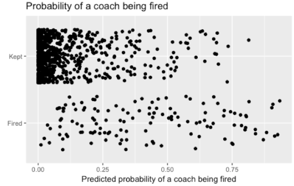
Altogether, the chart isn’t surprising. Most teams in most years aren’t firing their coach, and these teams are shown in the cluster of points in the top left of the graph. Meanwhile, teams that fire their coach tend to have predicted probabilities evenly spaced between 0 and 0.9.

The propensity score

At this point, we know we what suspected to begin with; the teams that fired their coach are, by and large, different from those that did not. This is a problem for most statistical tools. Basic comparisons like t-tests wouldn’t be able to account for these baseline differences, and even regression adjustment would be prone to bias given that the two groups (teams that fired their coaches and those that didn’t) are different from one another on several of the covariates that we would want to use in a model. Moreover, regression would be sensitive to model choice, and like most applications of statistics, the true model specification is unknown.

Here’s where causal inference comes in.

The probabilities depicted above are examples of propensity scores, defined as the conditional probability of receiving a treatment (in our case, of a team firing its coach). A nice property of propensity scores is that if two teams have the same propensity score, they also have, in expectation, the same distribution of observed covariates. This is really important. More technically, the distribution of covariates, conditional on the propensity score, is independent of whether or not a team chose to fire its coach.

The next critical part of propensity scores ties back to our potential outcome notation from earlier. Let’s assume that, conditional on the propensity score, the distribution of the set of potential outcomes is independent of our covariates, an assumption known as unconfoundedness. In other words, if I can find two teams with the same coach firing probability, where only one team actually fired its coach, the difference in those teams’ outcomes is an unbiased, unit-level estimate of firing a coach. Moreover, I can aggregate those differences across groups (say, every team that fired its coach) to provide an estimate of the causal effect of firing a coach (in this case, the benefit of firing a coach among teams that actually fired its coach).

These properties of propensity scores have made them widely applicable in fields like economics and government. There haven’t been many applications to sports, however, much to my chagrin.

Matching using the propensity score

The propensity score allows us to estimate the missing potential outcome that we don’t observe.

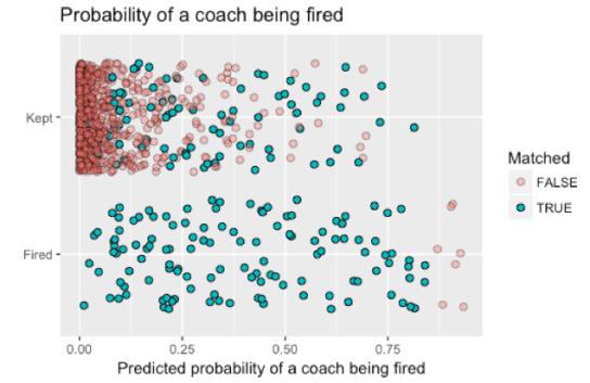
One way of doing this is to use matching, in which subjects receiving the treatment (those that fired a coach) are matched to those that didn’t. Using the Matching package in R, I matched teams that fired their coach to those that didn’t. Here’s the same plot as above, only now I use different colors (and shadings) to reflect observations that were and were not matched.

A few things to point out.

First, I used 1:1 matching with replacement, meaning that each coach who was fired (bottom row) was matched to one that didn’t (top row), but it was possible for coaches kept to be matched to more than one coach that was fired. Second, the set of coaches with a high probability of being fired who were actually fired (bottom right, in red) ended up not being part of my matched cohort. By and large, this is a good thing; there was no coach that was kept with a corresponding probability of being fired, and inference to this set of coaches would require extrapolation.

Checking covariate balance

But matching alone is not sufficient for inferring causes and effects. The next step is to make sure that the matching has done its job. Specifically, matching only works if the subjects matched to one another boast similar distributions of the observed covariates.

There are several ways to analyze covariate balance, and one of the more common ones compares the standardized bias for each covariate between each treatment group, done for both the pre and post-matched observations. Large value of standardized bias are bad – generally, the recommended cutoff for justifiable inference is 0.25 – and reflect groups that are not similar to one another.

Here are the pre and post-matched absolute standardized bias’ with our matched cohort.

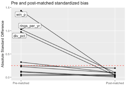
Each dot above reflects a variable from our logistic regression model (those recommended by Harrison and Mark). For example, the standardized bias of team win percentage (abbreviated as win_p) was roughly 1.5 in the pre-matched set of teams; after matching, the bias dropped below 0.15. In fact, the absolute standardized bias of all variables was sufficiently close to 0 after matching. This is a good thing; it entails that within our matched subset, teams that did and did not fire their coach are similar to one another (similar winning percentages, rings, GM changes, etc).

One important thing to point out is that the actual fit of the propensity score model is less important than the balance that is achieved: in other words, I’m worried less about things like collinearity and model fit statistics than I am about how similar the subjects matched to one another are. In our example, it looks like the teams that fired their coach and the ones that didn’t who ended up in our matched cohort are sufficiently alike.

 Analysis phase

Notice that I am yet to mention any observed, team-level outcome. This is not by accident; indeed, the above steps are considered to be the design phase of causal inference, done without looking at any outcome data.

The second step of causal inference is the analysis phase, in which the outcome of interest is contrasted within the matched cohort. For our purposes, I used the team’s winning percentage in the year following the firing or keeping of a coach.

There are a few reasonable approaches to to estimate the effect of coach firings on future winning percentage. One oft-recommended option is to use the combination of regression and matching together. Writes Stuart, “matching methods should not be seen in conflict with regression adjustment and in fact the two methods are complementary and best used in combination.”

With future team win percentage as my outcome, I fit a multivariate linear model with coach firing (yes/no) and 10 other predictors as covariates; these were the same 10 used by Glickman and Chase in their model of coach firings.

Turns out, not only is there no evidence that coach firing causes future success, if anything, it’s an inverse association. In our matched cohort, teams that kept their coach boasted a slightly higher (3.7%) winning percentage than those that fired their coach (p-value = 0.08). Notably, this estimate of 3.7% is relatively robust to model specification.

Extrapolating, our best estimate of the causal effect of firing a coach is about -0.6 wins in the following season, but given our uncertainty, it is unclear if this finding is due to chance or if there’s some true, net loss in the year following a coach firing. 

Discussion 

Hopefully this walk-through provides readers a rough introduction to how causal inference tools can be used, as well as the steps involved. You can repeat the analysis yourself using the code here, and if you are more familiar with causal tools, feel free to play around.

Some final thoughts:

• Those familiar with causal inference will notice I did not detail all of the assumptions required. One such assumption is positivity, which I think holds because it’s safe to assume that each team had a non-zero chance of firing its coach. Another is SUTVA, which I’m less confident about. As an example, it seems reasonable to argue that one teams’ choice to fire its coach ties into the potential outcomes of other teams.

• This post on visualizing covariate balance is really interesting, and would have saved me several hours of thesis writing. In fact, I wish I had seen it before I started writing the above post.

• You could certainly make the case that a team’s future win percentage in the year following a coach firing is not the best outcome. I chose the one-year outcome, as once you go to more than a year, things could get a bit dicey regarding our assumptions (i.e., if a team fires coaches in two consecutive years).

• If this were a more technical paper, I’d want to look at other variables related to the choice of firing a coach. As one example, a popular post-hoc tool in causal inference is sensitivity analysis, where some of the assumptions mentioned above are put to the test.